
Alexander Vladimirovich Markov | |
|---|---|
 Markov in 2020 | |
| Born | October 24, 1965 (age 58) Russia, Soviet Union |
| Education | Doctor of Science, Professor |
| Alma mater | Moscow State University (1987) |
| Scientific career | |
| Fields | Paleontology |
| Institutions | Moscow State University |
Alexander V. Markov (born October 24, 1965) is a Russian biologist, paleontologist, popularizer of science. Prize winner (2011) of the main Russian prize for popular science ("Prosvetitel"). [1]
Markov graduated from the Moscow State University (Faculty of Biology) in 1987. He has been working in the Paleontological Institute of the Russian Academy of Sciences since 1987. Doctor of biological sciences, Senior Research Professor of the Paleontological Institute, RAS. Professor of the RAS.
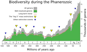
In collaboration with Andrey Korotayev he has demonstrated that a rather simple mathematical model can be developed to describe in a rather accurate way the macrotrends of biological evolution. They have shown that changes in biodiversity through the Phanerozoic correlate much better with hyperbolic model (widely used in demography and macrosociology) than with exponential and logistic models (traditionally used in population biology and extensively applied to fossil biodiversity as well). The latter models imply that changes in diversity are guided by a first-order positive feedback (more ancestors, more descendants) and/or a negative feedback arising from resource limitation. Hyperbolic model implies a second-order positive feedback. The hyperbolic pattern of the world population growth has been demonstrated by Korotayev to arise from a second-order positive feedback between the population size and the rate of technological growth. According to Markov and Korotayev, the hyperbolic character of biodiversity growth can be similarly accounted for by a feedback between the diversity and community structure complexity. They suggest that the similarity between the curves of biodiversity and human population probably comes from the fact that both are derived from the interference of the hyperbolic trend with cyclical and stochastic dynamics.[2][3]
YouTube Encyclopedic
-
1/3Views:29 0945 71748 172
-
Markov Chain Compression (Ep 3, Compressor Head)
-
Introductory tutorial on statistical sampling and MCMC (Alexander V. Mantzaris)
-
Markov Chain Matlab Tutorial--part 1
Transcription
Hey there trendy 30-something Silicon Valley resident, what you working on? Oh, a new app idea for mobile. That's pretty cool. So you've got your venture capital ready? Good, good. Fancy designer and website? Great. Man, I can't wait to see how your collaborative intelligent algorithm helps users find-- oh, you're not, you're not doing any of that. Oh well, you know I bet you've got a really cool compression algorithm. I mean, reducing your data transfer sizes to third world country-- no? Not doing that either, huh? Well, I mean are you doing anything with data compression? I mean, that's kind of important today. No, nothing huh? Well, hey listen. Don't get down on yourself. Come on, it's not that bad. I mean you can still fix it. All you need to do is take your recipe and sprinkle on a little bit of Markov chains and you'll be compressing data in no time. Well, you know Markov chains. The mathematical system that undergoes transitions from one state to another state on a state space and is generally characterized as memory-less. Such that the state depends only on the current state and not that of the sequence of events preceding it, providing that applications follow statistical models of real world processes. No? Nothing still? You know what? Maybe we should start from the beginning. But fret not, young Silicon Valley hipster. I'm here to help. My name is Colt McAnlis and this is Compressor Head. [THEME MUSIC] Teleprompter activate. [LAUGHTER] Now one of my favorite pastimes is actually taking great American traditions and distilling them into their state graph counterparts. Take example, baseball. Although it may seem like a bunch of random actions to have one team win or the other one lose, there's actually a very simple graph. Let's just look at a batter coming up to base. So the batter comes up to hit here. And there's really only two states. Number one, he can actually be out by hitting the ball or striking out or some other force of it. Or he can actually get on base. Now what the interesting part about this is that once you've move to either the on-base state or the out state, you actually return back and another batter comes up to bat. The cool thing about this is that it's pretty self-explanatory, right? Only three states and a couple transitions between them. Now what if we actually want to transmit some movement through this graph to another individual? Say for example, we have batter up, batter out, up, and then they get on base. Get up again and then another batter out. Well the simplest thing to do that we've been doing so far is assume that each state is a finite symbol. And we can encode each one with about two bits. Which means here we've got one, two, three, four, five six, at two bits per-- means if we want to send this to somebody, it'll be about 12 bits for the entire stream. However when we look at this, there may be a better way to do it. Now what if instead of assigning a variable bit lengths to each of its states, we instead actually assign bit codes to the transition between the states. So for example, we put a zero here, one here, zero here, and a zero here. Effectively, this allows us to encode the transitions between the states very differently, as long as the encoder and decoder know the states and how we're moving between them. Now if you take this set up here, that means that we're actually encoding these green arrows in our state. And this allows us to encode the entire stream in five bits, which is pretty good. But I think we can do better. If you look at our graph here, there's some implicit rules about baseball that we know to be true, that we don't actually have to encode in our graph. For example, when a batter is either out or on base, we know that another batter is going to come up no matter what. So we actually don't need to encode this in our stream. So we can get rid of this and get rid of this. Which means that the only information we really need to encode is whether or not when a better comes up, if they end up out or on base. This information allows us to encode all of our symbol data here in actually only three bits. So moving from 12 bits to 3 bits is actually pretty important. And what we've described here-- the ability to encode transitions rather than the exact states and then having some of the transitions be implicit in the encoder and decoder is actually the basis of how Markov encoding works. But of course, this is a simple example and it gets a little bit more tricky than this. In 1913, A.A. Markov found a new branch of probability theory by combining mathematics and poetry. Effectively delving into the text of an Alexander Pushkin novel, Markov spend hours sifting through patterns of vowels and consonants. And on January 23, 1913 publishers were detailing a statistical model that given a letter, it was a finite and reproducible probability associated with what letter would follow. You see by most accounts, Markov was a pretty meddlesome character, constantly involved with political feuds, public protests. He was fiercely competitive with any rivals in his field and actually spend a lot of time in jail for massive rounds of fisticuffs. How fitting is that the inventor of the algorithm, which is powering most of modern Silicon Valley, was a rebel without a cause. You see, Markov's concept o of probabilistic events selection was massively contrary to the world of statistics at the time, which mostly involves modeling count flipping and dice rolling. You see at its core, Markov chains help us answer questions about associative probability. For example, if it's cloudy today what are the chances that it's going to rain two days from now? A concept, which in 1913, was as predictable with mathematics as casting chicken bones. Think about that. Today Markov chains power some of the biggest and most complex big data algorithms in Silicon Valley. They're seen everywhere from cancer research to weather prediction to modeling consumer behavior and even figuring out what the best pizza joint is in San Jose. The best part is, we can use the same exact base algorithm that powers all these big things and use it for compression. Let's take a look. Channeling Markov's work, we can encode a given string by looking at a letter and noting the transition to the following letter. Now for the sake of simplicity here, I'm going to redraw the symbol pair transitions as a tree with the first letter in each pair resides the head of tree and the second pair resides as the child node. To give us some better terminology in this topic, we denote each pair in the context as a zero based order. That is the first letter of the pairs context zero, well the subsequent letters are context one. Now some of you graph purist may be looking at this graph and asking why T and N don't both point to O node as a child of context one. It is true that for both of these context zero symbols, O does follow as context one. But it's actually wrong to do that. Here's why. To understand why, let's re-encode the string with three simple steps, also known as second-order context. And use your concept of sharing the context one state. Now while this tree may look visually stunning and very pleasing it's actually quite inaccurate with respect to how the string is constructed. You see for example, this graph will allow you to move from T through O in context one, and then to T in context two, introducing the string TOT, which of course doesn't exist in the input data. This is of course an incorrect to the proper thing to do. And the proper thing to do is only chart context transition as unshared links. Now let's extend the concept forward a bit and take a look at a longer string using first-order contexts, that is two symbol pairs. You can see that a more real life example changes our distribution and gives us a different sort of tree for encoding with slightly more complex state relationships, with letters like T, O, and E have multiple potential transitions to the next context. If we wanted to encode this example, we would need some way to assign bits to each of the transitions between the context. The question, of course, is how many bits to assign to a transition, which we can determine as the max number of transitions from a node in the entire set. In this case, the O node in context zero has three transitions, which means we can use 2 bits for everything. Of course, this is a bit wasteful. For example, states with only one transition shouldn't need 2 bits. Plus, we need to keep around some number per node to let the decoder know how many bits to read. And what happens if there's 16 transitions per node instead of just 2? The correct answer here is to use variable length codes to describe transitions. This way, code words used to describe these transition can be variable in size and it can scale based upon what's actually needed. But remember, VLCs only work if you assign the most probable symbol the smallest code word. So in order to get the most efficient compression possible, we need to take probability into account when assigning code words, which thankfully is easy to do given the way we actually construct our chains. Doing so allows us to properly use VLCs to encode our data. And note one of the trickier parts about our scheme is that each context transition-- that is to say zero to each of its children in context one-- manage its own probability table. And as such, has its own VLC set. To be clear, you're not creating a VLC distribution across the entire graph. No, no. That would be madness. Recent years have seen the construction of truly enormous Markov chains. For example, page rank algorithm devised by Larry Page and Sergey Brin, the founders of Google, is based on a Markov chain whose states are the pages of the world wide web, perhaps 40 billion of them. The transitions between the states are actually links between the pages. The aim of the algorithm is to calculate for each page the probability that a reader following a link will randomly arrive at some further page. Now in order to make Markov practical for compression, we need to take a more technical look at the problem. Now when it comes to Markov chains, theory and practical implementations are night and day different. Sadly though this isn't something I can just talk about. No, we're actually going to have to get our hands dirty and encode some things to figure out what's going on. As efficient as Markov is for compression, it comes with one huge flaw. Let's say you want to transmit this encoding to the decoder. Well for each context transition or a parent to child transition, you'll need to store a frequency table-- that is the symbol and its frequency of incurrence. This data, of course, would need to be listed in the compressed streams so the decoder could properly decode this information. But even for this simple example, the overhead of this process is extreme. Just as for all of this frequency data, such that the decoder can properly work, we would need 53 bytes to this stream. The original stream is only 22 bytes, so obviously this is not helping. And it gets even worse the larger our data set is or the more context we decide to keep. The point here is that we can't simply transmit our percentages from the encoder to the decoder using the data stream. Instead we need to make the whole thing work as the decoder will generate the same statistical properties that the encoder is using for the data, as it's decoding the stream. Let's say we wanted to decode this stream, dynamically generate our probabilities, and Markov chain encode it all at the same time. We start out with a completely empty Markov data set. When we read the first letter, A, from the input stream, we need to encode it. But we can't because there's no data so far to use. As such, we need to start creating our tree. Once the trees is created, we need to encode A with a variable length code but we can't yet because we first need to assign it a probability. Since this is the first character we've seen, we can give it a probability of 100%. Once we have our probability, we can generate a Huffman tree, which will let us assign a code word to the symbol A. Since we've got nothing else in the tree, it gets the code word 0. Once we go to read our second letter, B, we also haven't seen it before. So we need to add it as a symbol and its probability to our tree. We also at this point need to update our probability for all the symbols in this context. Note that we've seen a second B, which updates its probability in the table and swaps its code word with A, which is exactly what we wanted since we're updating probabilities dynamically and generating variable length codes based on that. The best part is that we don't need to transmit the probabilities to the stream, just the encoded bits. However when we try to decode this, we run into a large problem, namely that we have no information about the literals or the probability table that was used to construct this bit stream, which basically means the decoder can't actually decode the stream and this is an incorrect encoding. To fix this, we're actually going to have to revisit our encoder and figure out a proper way to output literals so the decoder can consume them and reconstruct the original stream. Once we add A to the tree for the first time, we need some way of providing it to the output encoded stream so that the decoder can get it. To do this, we add a second output stream called the literal stream, which only contains 8 bits per symbol characters that we haven't actually seen yet. We now need to tell the output stream when it should read the explicit symbol from the literal stream, rather than expecting a variable length code. To do this, we introduced the concept of an escape code. An escape code is a special symbol that we're going to use in our probability table that allows the decoder to know when to read a full literal from our literal stream. Now an escape code is not a symbol in the sense that A, B, or C is but it does have residency in our probability table. So it will get a variable length code in the encoding. Rather than starting off with a blank tree, any new context nodes that are instead initialized with an escape code and set to 100% probability. When we read the letter A from the symbol stream, we add it to the context, update our code words, output an escape code to the bit stream, and then the letter A to the literal stream. Reading the letter B is the same process. We haven't seen it before. So we output the code word for an escape code and then a literal value. This is where the fun really starts to happen, kids. Once we read the next B, it's not a new symbol. We've actually seen it before. As such, it's critically important to note that when we're encoding an existing symbol that we output the variable length code before updating our stats and table code words. Once we update the probabilities of the table with the second B, the weights change the code word assignment. As such, the decoder wouldn't be able to see this type of change and it would break things. Decoding works the exact same way. Except when we encounter an escape code, it tells us to go read a symbol off the literal stream and output it. First we employ the process of reading variable length code from the bit stream. If you're not familiar with that, go check out Episode One. Since the only value we have is an escape code, we simply need to read a single bit from the stream and find that we're using an escape code. This tells us to go ahead and read 8 bits from the literal stream, push it to the output stream, and update our probability tables. We read the next zero from the bit stream and seeing that it's a variable length code as well, we know to read the next literal, output it, and update the probability tables. At this point, we have enough table information that the next 2 bits read off the bit stream match with the letter B, which of course we happily output. We've read A from the input stream and realized it's in the table. We've output our codes to the output bit stream and updated our probabilities. But because we're supporting context we need to actually create a new branch in the tree. In the naive solution, each symbol at each context level would contain a pointer to its children in the next context. But in order to make things work right, we have to start all subsequent context with an escape code. So the good news is that's the basics. However, the bad news is that we actually need to support a multi-context chain in order to get proper and legitimate compression. And in order to support that, we're going to revisit the encoder again and change how a few things work. Since we've just seen a new symbol at this context level that we haven't seen before, we need to start our chain back over again at context zero. Each time we read a symbol in context zero that already exists in the context, we move forward to read the next symbol operating in the subsequent context. So if the first two symbols were A, C, we would find the letter A and then add C to the first-order context set for encoding. And to be clear we treat a new symbol at any context as a completely new symbol. So if we encounter the series A, B, C in this encoding it's the first time that we've seen the letter C in context to following B. So we treat it the same way as we would with context zero by outputting it to the literal stream and emitting an escape code. Once this is entirely encoded, we take our final bit stream and literal stream and pass it along to whatever person on the internet wants it, without having to keep a single probability table around at all. In this solution the original stream was 88 bits while the encoded stream is only 46 bits, almost 50% reduction which isn't bad. So it should be really obvious at this point that efficient encoding of Markov chains has to strike a unique balance between the length of the chains that you need for compression and the available memory that you have on the system itself that you're running the encoder on. If you run out of memory early then it's not necessarily a good thing. A real encoder strike this balance with all separate profiles of system analysis memory and also writing additional context to disk to find the optimal solution. Now hopefully one of the questions you're asking yourself here is how do we properly adjusted the probability of an escape code when new symbols are added? In our little examples we did here, we simply subtracted hundredth of a point from it. But in reality it's not that simple. Unfortunately that's an entirely separate show that we're not going to cover today. In the mean time, Google it. Now some people view Markov chains as a step in an inevitable future where artificial intelligence algorithms run the entire gamut of data compression. And that's pretty easy to see. You see, keeping a multi-level context is much like tuning a neural network algorithm for artificial intelligence. Of course, we know by now those most successful Markov chains are actually terabytes of relational data long with thousands of context in two. Now lighter weight versions of Markov chains are already available today in modern compressors like 7-zip L pack and ZPack. It's easy to see a future down the road where artificial intelligence and cloud computing come together in some weird hybrid to create a revolution of data compression that we haven't seen it over 40 years. But that is a topic for a different show. My name is Colt McAnlis and this is Compressor Head. [THEME MUSIC]
References
- ^ {{http://www.vesti.ru/doc.html?id=641234&cid=7]}}
- ^ Markov, A.; Korotayev, A. (December 2007). "Phanerozoic marine biodiversity follows a hyperbolic trend". Palaeoworld. 16 (4): 311–318. doi:10.1016/j.palwor.2007.01.002.
- ^ Markov, A.; Korotayev, A. (2008). "Hyperbolic growth of marine and continental biodiversity through the Phanerozoic and community evolution". Journal of General Biology. 69 (3): 175–194. PMID 18677962.
Sources
- "Markov, Alexander V." Соционауки. Retrieved January 9, 2012.
| International | |
|---|---|
| National | |
| Academics | |